Learning the Backward Pass of FlashAttention
Part II Implementation in Triton
Recap Forward and Backward Passes of Standard Attention
In the first part of this tutorial, we have walked through a detailed derivation of formulas used in the backward pass of standard attention. For ease of reference, they are included as follows:
Given input sequences \(Q,\: K,\: V,\: \in \mathbb{R}^{N\times d}\) where \(N\) is the sequence length and \(d\) is the head dimension, the standard attention output \(O \in \mathbb{R}^{N\times d}\) is calculated as follows (forward pass):
\[S=QK^T \in \mathbb{R}^{N\times N}\quad P = \operatorname{softmax}(S) \quad O=PV \in \mathbb{R}^{N\times d}\]where \(\operatorname{softmax}\) is applied row-wise.
Then, assuming a scalar-valued loss function \(L\), by the backpropagation (i.e., reverse mode of automatic differentiation (AD)), the gradients of \(L\) w.r.t various inputs are calculated as follows:
\[\frac{\partial L}{\partial V} = P^T \frac{\partial L}{\partial O} \in \mathbb{R}^{N\times d}\] \[\frac{\partial L}{\partial P} = \frac{\partial L}{\partial O} V^T \in \mathbb{R}^{N\times N}\] \[\frac{\partial L}{\partial S} = \operatorname{dsoftmax}(\frac{\partial L}{\partial P}) \in \mathbb{R}^{N\times N}\] \[\frac{\partial L}{\partial Q} = \frac{\partial L}{\partial S}K \in \mathbb{R}^{N\times d}\] \[\frac{\partial L}{\partial K} = \frac{\partial L}{\partial S}^T Q \in \mathbb{R}^{N\times d}\]The Implementation of the Backward Pass of FlashAttention in Triton

To construct a direct correspondence between the mathematical equations and Triton code, we replace \(\frac{\partial L}{\partial V}\) with \(dV\) with a slight abuse of notation
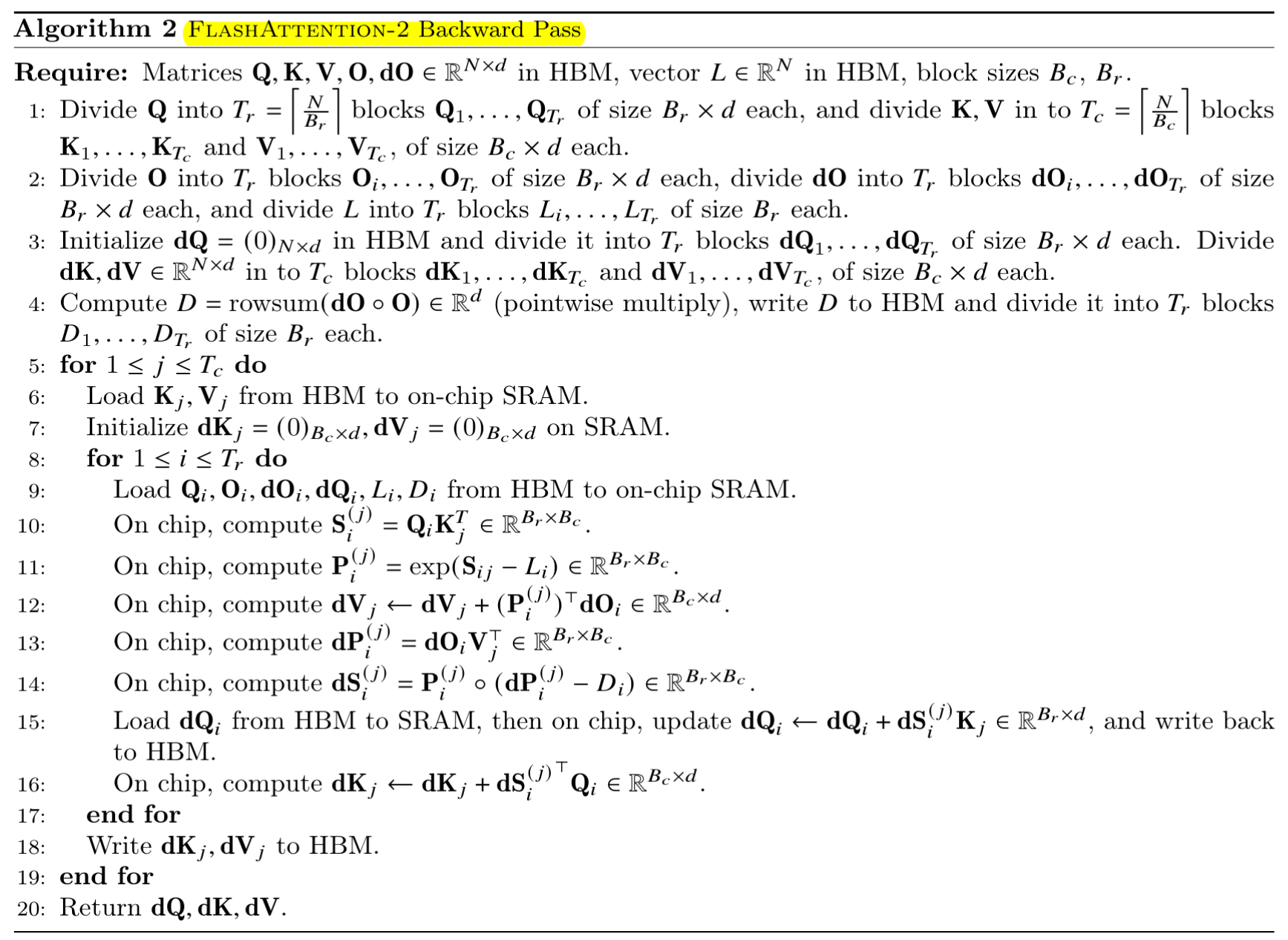
Another trick adopted in the FlashAttention paper
For self-containedness, it is included as follows, (Please note \(dS_{i,:}, dP_{i,:}\) are all column vectors):
\[dS_{i,:} = \operatorname{dsoftmax}dP_{i,:} = (\text{diag}(P_{i,:}) - P_{i,:}P_{i,:}^T)dP_{i,:} = P_{i,:} \circ dP_{i,:} - \left( P_{i,:}^T dP_{i,:} \right) P_{i,:}\]where \(\circ\) denotes Hadamard product (i.e., pointwise multiplication).
Recall that \(dP = dO V^T\), written in element-wise form, \(dP_{ij} = do_i^T v_j\), (Please note \(do_j, v_j, k_j\) here denote the j-th row of \(dO, V, K\) respectively, acting as a column vector.)
Now, we can define
\[D_i = P_{i,:}^T dP_{i,:} = \sum_j \frac{\exp(q_i^T k_j)}{L_i} do_i^T v_j = do_i^T \sum_j \frac{\exp(q_i^T k_j)}{L_i} v_j = do_i^T o_i\]then \(dS_{i,:} = P_{i,:} \circ dP_{i,:} - D_i P_{i,:}\).
Readers seeking a comprehensive treatment (e.g., the online-softmax trick in the forward pass) of FlashAttention are encouraged to refer to the original papers
Now, we are in a position to dive into the Triton implementation of the backward pass of FlashAttention2.
We assume readers have a basic familiarity with Triton. Otherwise, there are many excellent Triton tutorials, including the official ones, available online for your reference. In my view, figuring out how to move pointers to accurately access blocks of elements (i.e., load and store) in parallelly launched Triton programs is sufficient to grasp the core mechanisms of custom kernels developed in Triton.
Instead of using block pointer defined by make_block_ptr, I find that directly working with N-dimensional pointers to access elements in memory is more straightforward. Furthermore, mask and other are implicitly broadcast to pointer.shape when using N-dimensional pointers, which can be conveniently used to handle boundary conditions.
In the following, I will give some visual illustrations to facilitate your understanding of how tl.load() works, as there is no difference in read (tl.load()) and write (tl.store()) operations as long as their indexes are specified correctly.
  import numpy as np

  N = 8
  # Here, the content of the array is made intentionally to be the exact same as offsets relative to the base pointer.
  # Please note that in Triton language, all Pytorch tensors are implicitly converted to base pointers.

  A = np.arange(N * N).reshape(N, N)
  print(A)

  [[ 0  1  2  3  4  5  6  7]
   [ 8  9 10 11 12 13 14 15]
   [16 17 18 19 20 21 22 23]
   [24 25 26 27 28 29 30 31]
   [32 33 34 35 36 37 38 39]
   [40 41 42 43 44 45 46 47]
   [48 49 50 51 52 53 54 55]
   [56 57 58 59 60 61 62 63]]
  BLOCK_M = 2
  col_dim = N

  stride_row = N
  stride_col = 1

  offs_m = np.arange(BLOCK_M)[:, None] * stride_row + np.arange(col_dim)[None, :] * stride_col

  # N-dimensional tensors are stored contiguously in memory.
  # Otherwise, it would be recommended to call x.contiguous() before taking any tensor operations.
  # Here, we mimic this feature with np.ndarray.flatten.

  # illustrate loading tensors from memory
  print(A.flatten()[offs_m])

  [[ 0  1  2  3  4  5  6  7]
   [ 8  9 10 11 12 13 14 15]]
  # illustrate moving blocks `step_size` rows down, which will be used in the for loop to
  # traverse over one dimension of a tensor.
  step_size = 2
  print(A.flatten()[offs_m + step_size * N])

  [[16 17 18 19 20 21 22 23]
   [24 25 26 27 28 29 30 31]]
  # illustrate loading tensors directly in its transposed version and moving blocks accordingly
  offs_m_T = np.arange(BLOCK_M)[None, :] * stride_row + np.arange(col_dim)[:, None] * stride_col
  print(A.flatten()[offs_m_T])
  print(A.flatten()[offs_m_T + step_size * N])

  [[ 0  8]
   [ 1  9]
   [ 2 10]
   [ 3 11]
   [ 4 12]
   [ 5 13]
   [ 6 14]
   [ 7 15]]

  [[16 24]
   [17 25]
   [18 26]
   [19 27]
   [20 28]
   [21 29]
   [22 30]
   [23 31]]
Here, we analyse a simplified version of FlashAttention (technically, FlashAttention2) adapted from the official Triton tutorial Fused Attention, accounting for both the ‘Causal’ and ‘Non-Causal’ modes.
The implementation of the backward pass of FlashAttention can be generally grouped into three stages:
-
Calculate the matrix \(D\) first as a preprocessing step, where \(D_i = do_i^T o_i\), which corresponds to the variable
delta = torch.empty_like(M). Its size is(Batch, Num_Heads, N_CTX), and is realised in the function_attn_bwd_preprocess(). -
Calculate \(dV, dK\) via the function
_attn_bwd_dkdv(). -
Calculate \(dQ\) via the function
_attn_bwd_dq().
  @triton.jit
  def _attn_bwd_preprocess(O, DO,  #
                           Delta,  #
                           Z, H, N_CTX,  #
                           BLOCK_M: tl.constexpr, HEAD_DIM: tl.constexpr  #
                           ):
      off_m = tl.program_id(0) * BLOCK_M + tl.arange(0, BLOCK_M)
      off_hz = tl.program_id(1)
      off_n = tl.arange(0, HEAD_DIM)
      # load
      o = tl.load(O + off_hz * HEAD_DIM * N_CTX + off_m[:, None] * HEAD_DIM + off_n[None, :]).to(tl.float32)
      do = tl.load(DO + off_hz * HEAD_DIM * N_CTX + off_m[:, None] * HEAD_DIM + off_n[None, :]).to(tl.float32)
      delta = tl.sum(o * do, axis=1)
      tl.store(Delta + off_hz * N_CTX + off_m, delta)
where delta = tl.sum(o * do, axis=1) implements the equation \(D_i = do_i^T o_i\).
To calculate \(dV, dK\), a block of elements of k, v is first loaded (sequence parallelisation), and then carries out a loop over the length dimension of q.
  start_n = pid * BLOCK_N1
  offs_n = start_n + tl.arange(0, BLOCK_N1)
  # load K and V: they stay in SRAM throughout the inner loop.
  k = tl.load(K + offs_n[:, None] * stride_tok + offs_k[None, :] * stride_d)
  v = tl.load(V + offs_n[:, None] * stride_tok + offs_k[None, :] * stride_d)
For the non-causal case, it is straightforward,
  start_m = 0
  num_steps = (N_CTX - start_m) // BLOCK_M1

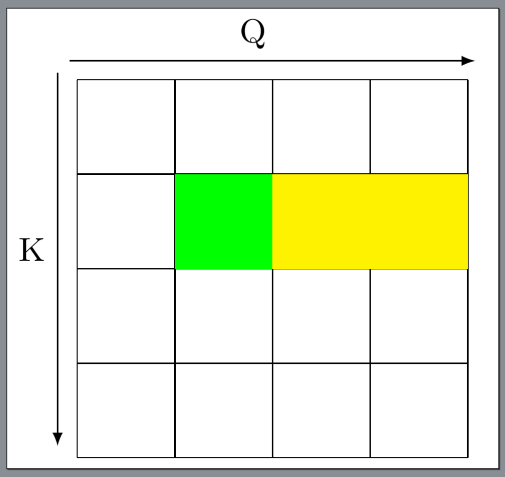
For the causal case (please note that causal modelling is only used in self-attention), the procedure is split into two steps:
- Calculate the non-masked blocks (yellow squares in the Fig-1) by only changing
start_m = start_n + BLOCK_N1. -
Calculate the diagonal block (the green square in the Fig-1) by setting
  start_m = start_n
  MASK_BLOCK_M1: tl.constexpr = BLOCK_M1 // BLK_SLICE_FACTOR
  num_steps = BLOCK_N1 // MASK_BLOCK_M1
  # The main inner-loop logic for computing dK and dV.
  @triton.jit
  def _attn_bwd_dkdv(dk, dv,  #
                     Q, k, v, sm_scale,  #
                     DO,  #
                     M, D,  #
                     # shared by Q/K/V/DO.
                     stride_tok, stride_d,  #
                     H, N_CTX, BLOCK_M1: tl.constexpr,  #
                     BLOCK_N1: tl.constexpr,  #
                     HEAD_DIM: tl.constexpr,  #
                     # Filled in by the wrapper.
                     start_n, start_m, num_steps,  #
                     MASK: tl.constexpr):
      offs_m = start_m + tl.arange(0, BLOCK_M1)
      offs_n = start_n + tl.arange(0, BLOCK_N1)
      offs_k = tl.arange(0, HEAD_DIM)
      qT_ptrs = Q + offs_m[None, :] * stride_tok + offs_k[:, None] * stride_d
      do_ptrs = DO + offs_m[:, None] * stride_tok + offs_k[None, :] * stride_d
      # BLOCK_N1 must be a multiple of BLOCK_M1, otherwise the code wouldn't work.
      tl.static_assert(BLOCK_N1 % BLOCK_M1 == 0)
      curr_m = start_m
      step_m = BLOCK_M1
      for blk_idx in range(num_steps):
          qT = tl.load(qT_ptrs)
          # Load m before computing qk to reduce pipeline stall.
          offs_m = curr_m + tl.arange(0, BLOCK_M1)
          m = tl.load(M + offs_m)
          sT = tl.dot(k, qT)
          pT = tl.math.exp2(sT - m[None, :])
          # Autoregressive masking.
          if MASK:
              mask = (offs_m[None, :] >= offs_n[:, None])
              pT = tl.where(mask, pT, 0.0)
          do = tl.load(do_ptrs)
          # Compute dV.
          ppT = pT
          ppT = ppT.to(tl.float16)
          dv += tl.dot(ppT, do)
          # D (= delta) is pre-divided by ds_scale.
          Di = tl.load(D + offs_m)
          # Compute dP and dS.
          dpT = tl.dot(v, tl.trans(do)).to(tl.float32)
          dsT = pT * (dpT - Di[None, :])
          dsT = dsT.to(tl.float16)
          dk += tl.dot(dsT, tl.trans(qT))
          # Increment pointers.
          curr_m += step_m
          qT_ptrs += step_m * stride_tok
          do_ptrs += step_m * stride_tok
      return dk, dv
  qT = tl.load(qT_ptrs)
  # Load m before computing qk to reduce pipeline stall.
  offs_m = curr_m + tl.arange(0, BLOCK_M1)
  m = tl.load(M + offs_m)
  sT = tl.dot(k, qT)
  pT = tl.math.exp2(sT - m[None, :])
This part of code recomputes \(S = QK^T\) and \(P = \operatorname{softmax}(S)\) (actually its transposed version, and therefore it needs to pay attention to the broadcast rule m[None, :]. m is stored in the forward pass for calculating softmax in a numerical stable manner.).
dv += tl.dot(ppT, do) implements the equation \(dV = P^T dO\). As the calculation \(dv_j = \sum_i P_{ij} do_i\), where \(dv_j, do_i\) denote the j-th and i-th row of \(V, O\) respectively, is chunked into multiple blocks, so do not forget the accumulation sum.
dpT = tl.dot(v, tl.trans(do)).to(tl.float32) implements the equation \(dP = dO V^T\) (its transposed version).
dsT = pT * (dpT - Di[None, :]) implements the equation \(dS = \operatorname{dsoftmax}(dP) \in \mathbb{R}^{N\times N}\), which is further simplified to
as discussed above (its transposed version).
dk += tl.dot(dsT, tl.trans(qT)) implements the equation \(dK = dS^T Q\).
\(dQ\) is calculated similarly: a block of elements of q is first loaded (sequence parallelisation), and then carries out a loop over the length dimension of k, v.
  start_m = pid * BLOCK_M2
  offs_m = start_m + tl.arange(0, BLOCK_M2)
  # load q, do, m and Di: they stay in SRAM throughout the inner loop.
  q = tl.load(Q + offs_m[:, None] * stride_tok + offs_k[None, :] * stride_d)
  do = tl.load(DO + offs_m[:, None] * stride_tok + offs_k[None, :] * stride_d)

  m = tl.load(M + offs_m)
  m = m[:, None]

  Di = tl.load(D + offs_m)
  Di = Di[:, None]

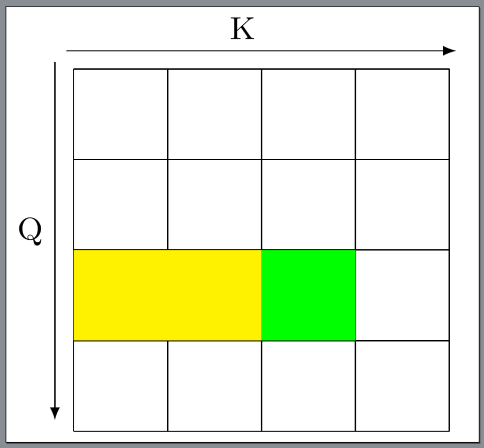
For the causal case, the procedure is split into two steps:
- Calculate the non-masked blocks (yellow squares in the Fig-2) by setting
end_n = start_mnum_steps = end_n // BLOCK_N2. So in the inner loop overk, v, the start and end indexes are0andstart_m, respectively. -
Calculate the diagonal block (the green square in the Fig-2) by setting
  MASK_BLOCK_N2: tl.constexpr = BLOCK_N2 // BLK_SLICE_FACTOR
  num_steps = BLOCK_M2 // MASK_BLOCK_N2
And the start and end indexes are
start_mandstart_m + BLOCK_M2respectively.
For the non-causal case, in the inner loop over k, v, the start and end indexes are simply 0 and N_CTX, respectively. However, in my implementation, it is also split into two steps: 1) from 0 to start_m, and 2) from start_m to N_CTX.
  @triton.jit
  def _attn_bwd_dq(dq, q, K, V,  #
                   do, m, Di,
                   # shared by Q/K/V/DO.
                   stride_tok, stride_d,  #
                   H, N_CTX,  #
                   BLOCK_M2: tl.constexpr,  #
                   BLOCK_N2: tl.constexpr,  #
                   HEAD_DIM: tl.constexpr,  #
                   # Filled in by the wrapper.
                   start_m, start_n, num_steps,  #
                   MASK: tl.constexpr):
      offs_m = start_m + tl.arange(0, BLOCK_M2)
      offs_n = start_n + tl.arange(0, BLOCK_N2)
      offs_k = tl.arange(0, HEAD_DIM)
      kT_ptrs = K + offs_n[None, :] * stride_tok + offs_k[:, None] * stride_d
      vT_ptrs = V + offs_n[None, :] * stride_tok + offs_k[:, None] * stride_d
      # BLOCK_M2 must be a multiple of BLOCK_N2, otherwise the code wouldn't work.
      tl.static_assert(BLOCK_M2 % BLOCK_N2 == 0)
      curr_n = start_n
      step_n = BLOCK_N2
      for blk_idx in range(num_steps):
          kT = tl.load(kT_ptrs)
          vT = tl.load(vT_ptrs)
          s = tl.dot(q, kT)
          p = tl.math.exp2(s - m)
          # Autoregressive masking.
          if MASK:
              offs_n = curr_n + tl.arange(0, BLOCK_N2)
              mask = (offs_m[:, None] >= offs_n[None, :])
              p = tl.where(mask, p, 0.0)
          # Compute dP and dS.
          dp = tl.dot(do, vT).to(tl.float32)
          ds = p * (dp - Di)
          ds = ds.to(tl.float16)
          # Compute dQ.
          # NOTE: We need to de-scale dq in the end, because kT was pre-scaled.
          dq += tl.dot(ds, tl.trans(kT))
          # Increment pointers.
          curr_n += step_n
          kT_ptrs += step_n * stride_tok
          vT_ptrs += step_n * stride_tok
      return dq
  kT = tl.load(kT_ptrs)
  vT = tl.load(vT_ptrs)
  s = tl.dot(q, kT)
  p = tl.math.exp2(s - m)
This part of code recomputes \(S = QK^T\) and \(P = \operatorname{softmax}(S)\).
dp = tl.dot(do, vT).to(tl.float32) implements the equation \(dP = dO V^T\).
ds = p * (dp - Di) implements the equation \(dS_{i,:} = P_{i,:} \circ dP_{i,:} - D_i P_{i,:}\).
dq += tl.dot(ds, tl.trans(kT)) implements the equation \(dQ = dS K\).
Concluding Remarks
Voila! We have walked through the core implementation of the backward pass of FlashAttention, where the Triton code shares a high similarity with matrix calculus equations. You can check out the Github repo Learning-to-Learn-DL containing an IPython notebook which is supposed to offer a more enhanced interactive experience and another notebook where a more flexible implementation of FlashAttention2 is given, which can handle both self-attention and cross-attention with arbitrary lengths. However, for practical usage, I recommend using the official FlashAttention Repo written in CUDA. Furthermore, I believe this post will facilitate your understanding of the Triton implementation given in the official FlashAttention Repo.
@misc{Cai2025flashattnbackward-2,
    author = {Xin Cai},
    title = {Learning the Backward Pass of FlashAttention: Part II Implementation in Triton},
    howpublished = {\url{https://totalvariation.github.io/blog/2025/intro-flashattention-backward-part2/},
    note = {Accessed: 2025-07-21},
    year = {2025}
}